Probability and statistics: the concepts worth being precise about

Ask ten people what a 70% chance of rain means and you’ll get at least three answers. That’s not a failure of arithmetic. It’s that probability has more than one definition, and which one you’re using changes what the number is claiming.

Introduction

This is the first part of a short series on the statistics you actually need before any of the modelling makes sense. Not a course. More the set of ideas I find myself re-explaining most often, with the pictures I’d draw on a whiteboard.

We’ll start with the three ways of defining probability and why they disagree, then work through the rules that let you combine events, then the descriptive statistics that summarise a sample. Every plot is generated by R code you can run, and the code is in the post.

Probability Fundamentals

Probability quantifies how likely something is. That much everyone agrees on. Where it gets interesting is what the number is measuring, and there are three different answers.

I. Definitions:

• Experiment: An action or procedure that results in one of several possible outcomes. For example, rolling a die is an experiment with six possible outcomes (1, 2, 3, 4, 5, or 6).
• Outcome: The result of an experiment. In the die-rolling example, if the die lands on 3, then the outcome is 3.
• Event: A set of one or more outcomes. In the die-rolling example, an event could be the die showing an even number, which includes the outcomes 6.
• Sample Space: The set of all possible outcomes of an experiment. For the die-rolling example, the sample space is 6.

II. Types of Probability:

• Classical: Based on the assumption that all outcomes are equally likely. In the die-rolling example, the classical probability of getting an even number is 1/2 (3 even numbers out of 6 possible outcomes).
• Relative Frequency: Based on the observed frequencies of outcomes in a sample. For instance, suppose we roll a die 100 times and observe 40 even numbers. The relative frequency of getting an even number is 40/100 = 0.4.
• Subjective: Based on an individual’s personal judgment or belief. A person may believe that it is more likely to rain tomorrow based on their interpretation of weather patterns and past experiences, even if objective data suggests otherwise.

Let’s use a real-world dataset to illustrate the relative frequency approach. We will analyze the number of cylinders in vehicles from the mtcars dataset, which is included in R. We will calculate the relative frequency of vehicles with 4, 6, and 8 cylinders.

library(knitr)
data(mtcars)

cylinder_counts <- mtcars %>% count(cyl)
total_cars <- sum(cylinder_counts$n)
relative_frequencies <- cylinder_counts %>% 
mutate(relative_frequency = n / total_cars)

kable(relative_frequencies, caption = "Relative Frequencies of Cylinder Counts in Vehicles")

Relative Frequencies of Cylinder Counts in Vehicles

In the table above, the “cyl” column represents the number of cylinders in a vehicle, the “n” column shows the count of vehicles with the corresponding number of cylinders, and the “relative_frequency” column displays the relative frequency of each cylinder count in the dataset.

Here’s the table rendered as a chart — the original output from this post’s code:

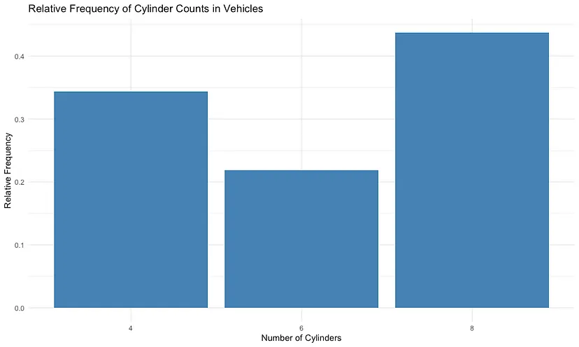
Now, the ggplot2 code that draws it:

library(tidyverse)

ggplot(relative_frequencies, aes(x = factor(cyl), y = relative_frequency)) +
  geom_col(fill = "steelblue") +
  labs(title = "Relative Frequency of Cylinder Counts in Vehicles",
       x = "Number of Cylinders",
       y = "Relative Frequency") +
  theme_minimal()

Simulation is the quickest way to see the relative-frequency idea work. Roll a fair die a few times and the proportions are all over the place; roll it ten thousand times and they settle near a sixth. Watch how fast that happens.

set.seed(42) # Set seed for reproducibility
n_rolls <- 1000
die_rolls <- sample(1:6, size = n_rolls, replace = TRUE)

die_rolls_df <- data.frame(outcome = die_rolls) %>%
  count(outcome) %>%
  mutate(relative_frequency = n / n_rolls)

die_rolls_df

This will generate a data frame with the outcome, count, and relative frequency of each die roll:

Now, let’s create a bar chart to visualize the relative frequencies:

ggplot(die_rolls_df, aes(x = factor(outcome), y = relative_frequency)) +
  geom_col(fill = "steelblue") +
  labs(title = "Die Roll Simulation",
       x = "Outcome",
       y = "Relative Frequency") +
  theme_minimal()

And here’s what came out of that run:

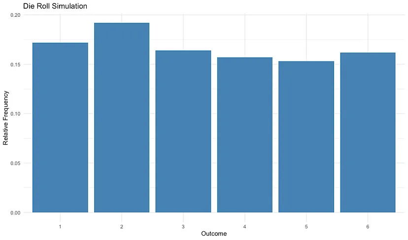
Six outcomes, ten thousand rolls, and every bar hovers near one-sixth without any of them landing exactly there. That wobble is the point: relative frequency converges on the classical answer, and never quite equals it at any finite number of rolls.

III. Probability Rules:

Addition Rule: The addition rule helps us calculate the probability of either event A or event B (or both) occurring. The rule is defined as:

P(A ∪ B) = P(A) + P(B) − P(A ∩ B)

Here, P(A ∪ B) represents the probability of event A or event B occurring, while P(A ∩ B) denotes the probability of both events A and B happening together.

Example: Suppose we have a deck of 52 playing cards. What is the probability of drawing either a red card (hearts or diamonds) or a queen?

There are 26 red cards and 4 queens in the deck, but 2 of the queens are also red cards (queen of hearts and queen of diamonds). So, applying the addition rule:

P(Red ∪ Queen) = P(Red) + P(Queen) − P(Red ∩ Queen)
P(Red ∪ Queen) = (26/52) + (4/52) − (2/52) = 28/52 ≈ 0.5385

Multiplication Rule: The multiplication rule helps us determine the probability of both events A and B occurring simultaneously. The rule is defined as:

P(A ∩ B) = P(A|B) * P(B)

Here, P(A|B) represents the probability of event A occurring given that event B has occurred.

Example: Consider a bag containing 5 blue and 3 red balls. We draw two balls from the bag without replacement. What is the probability of drawing a blue ball first, followed by a red ball?

To apply the multiplication rule, we first calculate the probability of each event:

P(Blue1) = 5/8 P(Red2|Blue1) = 3/7

Now, we can compute the probability of both events happening together:

P(Blue1 ∩ Red2) = P(Blue1) * P(Red2|Blue1) = (5/8) * (3/7) ≈ 0.2679

In the next part of this series, we will cover topics related to Descriptive Statistics.

For more practical tips and insights on AI, data science, and statistics, explore our blog at Analytica Data Science Solutions. Discover engaging content to expand your knowledge and stay up-to-date with the latest developments.

In this blog post, we have covered the basics of probability and statistics. If you wish to further expand your knowledge and understanding, here are some references to help you dive deeper into these topics:

Books:

1. DeGroot, M. H., & Schervish, M. J. (2012). Probability and Statistics (4th ed.). Pearson.
2. Wackerly, D., Mendenhall, W., & Scheaffer, R. L. (2007). Mathematical Statistics with Applications (7th ed.). Cengage Learning.
3. Casella, G., & Berger, R. L. (2001). Statistical Inference (2nd ed.). Duxbury Press.
4. Hastie, T., Tibshirani, R., & Friedman, J. (2009). The Elements of Statistical Learning: Data Mining, Inference, and Prediction (2nd ed.). Springer.
5. Wickham, H., & Grolemund, G. (2016). R for Data Science: Import, Tidy, Transform, Visualize, and Model Data. O’Reilly Media.

Websites:

1. Khan Academy: Probability and Statistics: https://www.khanacademy.org/math/statistics-probability
2. Stat Trek: Teach yourself statistics: https://stattrek.com/
3. Carnegie Mellon University Probability & Statistics: https://oli.cmu.edu/courses/probability-statistics-open-free/

Online Courses:

1. Coursera: Statistics with R Specialization by Duke University: https://www.coursera.org/specializations/statistics
2. Coursera: Introduction to Probability and Data with R by Duke University: https://www.coursera.org/learn/probability-intro
3. edX: Probability and Statistics in Data Science using Python by the University of California, San Diego: https://www.edx.org/course/probability-and-statistics-in-data-science-using-python
4. DataCamp: Introduction to Probability in R: https://www.datacamp.com/courses/introduction-to-probability-in-r
5. DataCamp: Foundations of Probability in R: https://www.datacamp.com/courses/foundations-of-probability-in-r